All posts by CaAl

NWO, Discriminatie en de Simpsonparadox

22/09/2015 CaAl 19 Comments

Begin jaren ’70 was er ophef in de media: de Universiteit van Californië in Berkeley discrimineerde bij het toelaten van studenten. De toelatingscijfers van 1973 waren duidelijk:

	Aantal kandidaten	Toegelaten
Mannen	8442	44%
Vrouwen	4321	35%

Mannen worden vaker toegelaten dan vrouwen. Met een statistische toets is na te gaan of deze cijfers niet gewoon toeval hadden kunnen zijn. Er zijn verschillende toetsen die geschikt zijn voor dit soort analyses (de een wat geschikter dan de ander), zoals de chi-kwadraat toets (eventueel met continuïteitscorrectie) of de exacte toets van Fisher. Welke geschikte toets je ook neemt, het antwoord is duidelijk: de kans dat deze vrouwonvriendelijke resultaten het gevolg van toeval zijn is verwaarloosbaar klein: kleiner dan 1 op een miljard.

Een rechtzaak volgde vanwege dit overduidelijk geval van discriminatie. Een team van statistici uit Berkeley, onder leiding van Peter Bickel, besloot de data nader te bestuderen. Hun conclusie, beschreven in het paper “Sex Bias in Graduate Admissions: Data from Berkeley” (paywall) in Science, is duidelijk: er is helemaal geen sprake van discriminatie.

Wat was het geval? Vrouwen bleken zich, in het algemeen, aan te melden voor studies waarbij een lager toelatingspercentage gold vergeleken bij de studies die voor mannen populair waren. Zo was er een faculteit (faculteit ‘B’ noemt Wikipedia deze; ik kan de data van Bickel et al zelf ook niet inzien vanwege de paywall) waar bijna twee-derde van de aanmeldingen gehonoreerd werden, terwijl bij een andere faculteit (‘E’) slechts een kwart werd toegelaten. En wat bleek: de toegankelijke faculteit B was veel populairder bij mannen (560 aanmeldingen) dan bij vrouwen (25 aanmeldingen) terwijl de strenge faculteit E twee keer zo veel vrouwen (393 stuks) als mannen (191 stuks) moest beoordelen. Indien rekening gehouden werd met de verschillen in strengheid van de verschillende faculteiten, verdween de discriminatie volledig. (Sterker nog: bij vier van de zes faculteit lag het toelatingspercentage van vrouwen hoger dan dat van mannen).

Dit fenomeen staat bekend als de Simpsonparadox, vernoemd naar de Britse statisticus Edward Simpson die in 1951 een paper getiteld “The Interpretation of Interaction in Contingency Tables” publiceerde (semi-paywall). Dit femomeen is breed bekend.

Tot zo ver de jaren ’70. September 2015 was er ophef in de (sociale) media: NWO discrimineert bij het toekennen van onderzoeksbeurzen. In opdracht van NWO zelf, hebben Leidse psychologen Romy van der Lee en Naomi Ellemers zich verdiept in de door NWO toegekende subsidies van de rondes van het VENI-subsidieschema uit 2010-2012. Hun paper “Gender contributes to personal research funding success in The Netherlands” (paywall, maar het ‘supplementary material’ is dan weer wel gratis) verscheen onlangs in PNAS. De cijfers zijn duidelijk:

	Aantal Beursaanvragen	toegekend
Mannen	1635	17,7%
Vrouwen	1188	14,9%

De cijfers zijn wellicht niet zo overduidelijk als die van het voorbeeld uit Berkeley, maar mannen krijgen inderdaad relatief vaker een beurs toegekend. De auteurs zelf schrijven “The success rate was systematically lower for female applicants than for male applicants [14.9% vs. 17.7%; χ²(1) = 4.01, P = 0.045, Cramer’s V = 0.04]”. De p-waarde zit nèt onder de magische 5%-grens, dus het is significant, dus het is bewezen: NWO discrimineert! Althans, dat was de strekking van de krantenkoppen. Maar zo simpel ligt het niet. Op de hier gebruikte methodiek kom ik onderaan deze post nog terug, maar mijn hoofdbezwaar is dat hier ook duidelijk sprake is van de Simpsonparadox.

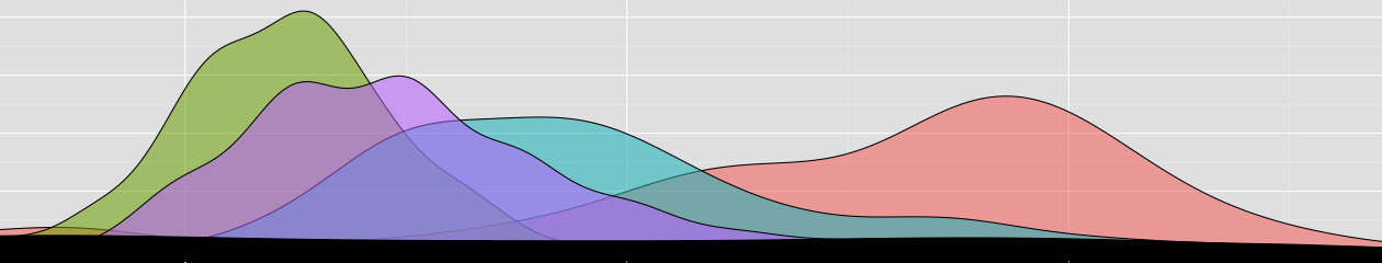
In de online tabel zijn de toekenningspercentages uitgesplitst naar de 9 verschillende onderzoeksprogramma’s van NWO. En wat blijkt: er is zowel een enorm verschil in het aandeel van vrouwen bij de aanvragen per programma (variërend van 11% tot 51%) als een enorm verschil in honoreringskans per programma (variërend van 13% tot 26%):

Relatie percentage vrouwelijke aanvragers (horizontaal) en honoreringskans (verticaal) — Relatie percentage vrouwelijke aanvragers (horizontaal) en totale honoreringskans (mannen & vrouwen gezamenlijk) (verticaal)

Het aandeel vrouwelijke aanvragers is het hoogst bij ZonMW (gezondheidswetenschappen) en MaGW (Maatschappij- en Gedragswetenschappen) en dit zijn precies de twee programma’s met de slechtste honoreringskans. Het aandeel vrouwelijke aanvragers is het laagst bij Natuurkunde (een bedroevende 11%), het programma met de hoogste honoreringskans.

Van de negen programma’s zijn er vier waarbij vrouwen een hoger honoreringspercentage hebben dan mannen: Exacte wetenschappen, Geesteswetenschappen, ‘Technologiestichting STW’ en ‘Gebiedsoverschreidend’. Bij de overige vijf programma’s, Scheikunde, Natuurkunde, Aard- en Levenswetenschappen, MaGW en ZonMW, halen mannen net betere resultaten. In geen der gebieden is het verschil zodanig dat – ermee rekening houdend dat meervoudige toetsen worden uitgevoerd – het verschil significant genoemd kan worden.

Oftewel: het discriminatievermoeden wordt in dit geval niet zo extreem sterk onderuit gehaald als in het klassieke voorbeeld uit Berkeley, maar wel sterk genoeg om te zien dat er niet geconcludeerd kan worden, op basis van deze data, dat er sprake is van discriminatie. NB: het tegendeel – er is geen sprake van discriminatie – kan ook niet geconcludeerd worden. De enige conclusie is dat uit de cijfers geen solide conclusie te trekken valt.

Tot zover de Simpsonparadox bij de NWO-cijfers. Nog enkele andere opmerkingen:

1) De cijfers per NWO-programma duiden naar mijn mening wel op een vorm van geïnstitutionaliseerde discriminatie: in geen van de negen onderzoeksprogramma’s vormen vrouwen de duidelijke meerderheid terwijl er in vier van de negen programma’s minstens twee keer zo veel mannen een aanvraag doen als vrouwen. Dit zijn nog steeds de bètarichtingen als scheikunde, natuurkunde, exacte wetenschappen en technologie (STW). Maar die vorm van discriminatie valt NWO niet (direct) aan te rekenen: dat is een maatschappelijk probleem dat op alle niveaus aangepakt moet worden. Het land heeft meer Ionicas Smeets, Ashas ten Broeke, Hannahs Fry en genderneutraal voedsel nodig, maar de rol die NWO daarin kan spelen is beperkt.

2) Ik zou nog terugkomen op de zin “The success rate was systematically lower for female applicants than for male applicants [14.9% vs. 17.7%; χ²(1) = 4.01, P = 0.045, Cramer’s V = 0.04]”. Bij deze. De chi-kwadraattoets is niet de meest geschikte toets om toe te passen bij 2×2 tabellen met frequenties. Dit omdat de chi-kwadraat een zogenaamde asymptotische toets is: hoe kleiner de frequenties in de tabel, hoe onnauwkeuriger de data. Een veelgebruikte correctie die die onnauwkeurigheid deels weghaalt, is die van Yates. Als je die toepast, verandert de p-waarde minimaal (want we werken hier met best grote frequenties): van 0,045 naar 0,051. Het verschil is minimaal, maar het springt wel nèt over de magische 5%. Als je met grote stelligheid een p-waarde vlak onder 5% als een duidelijk effect presenteert, zou je met dezelfde stelligheid een p-waarde daar vlak boven als “geen effect gevonden” moeten afdoen. Een ander alternatief – en beter omdat het geen asymptotische benadering is – is de exacte toets van Fisher. Deze geeft p = 0,046 (hoera! net aan de significante kant!). Er is eigenlijk geen enkele reden om de Fishertoets niet te gebruiken. Het enige nadeel is dat deze computationeel veel zwaarder is dan de chi-kwadraat toets. Dat was een terecht nadeel in de jaren ’20, toen Fisher die test ontwikkelde en Turing de moderne computer nog niet had uitgevonden. Anno 2015, kost de Fishertoets op deze data mijn computer 3 milliseconden.

3) Niet alleen is de p-waarde net wel/net niet significant, de effectgrootte is minimaal: Cramer’s V was gelijk aan 0,04. Als er al een verschil zou zijn tussen toelatingskansen van mannen en vrouwen, dan zou dit verschil erg klein zijn. Een klein beetje discriminatie is natuurlijk nog steeds ongewenst, maar de combinatie van minieme effectgrootte en nauwelijks significante p-waarde vereisen een veel voorzichtigere conclusie dan de conclusie “The data reported herein provide compelling evidence of gender bias in personal grant applications to obtain research funding.” van Van der Lee en Ellemers. (Hierbij moet wel opgemerkt worden dat de auteurs nog andere zaken bekeken dan alleen de 2×2 tabel die ik hier besproken heb. Maar ook met die extra gegevens is er geen statistische aanleiding tot grootspraak.)

4) De auteurs hebben de VENI-data van 2010, 2011 en 2012 bekeken. We zijn inmiddels alweer even verder. Zo kregen in 2015 14,9% van de vrouwen en ‘slechts’ 13,9% van de mannen de door hun gewenste beurs. Zou dit jaar bij de analyse betrokken zijn dan was – zelfs met de oppervlakkige chi-kwadraattoets die Van der Lee en Ellemers hebben toegepast – er niks overgebleven van de significante resultaten.

5) Los van de discussie over discriminatie laten de cijfers wel een schokkend iets zien: zowel voor mannen als voor vrouwen is het honoreringspercentage extreem laag. Dit houdt in dat er jaarlijks honderden wetenschappers zijn die enkele maanden van hun academisch leven besteden aan het schrijven van een voorstel dat uiteindelijk de prullenbak in gaat. Daar gaan dus duizenden en duizenden manuren èn vrouwuren aan verloren. Inmiddels wijst onderzoek na onderzoek uit dat de huidige manier van wetenschappelijke subsidies mogelijk meer nadelen dan voordelen heeft.

6) Deze hele discussie kent wat nare kanten – zo komen er wéér twee sociaal psychologen in het nieuws vanwege rammelend statistisch onderzoek – maar kan mogelijk ook tot goede ontwikkelingen leiden: zoals Daniël Lakens en Rolf Hut vandaag al in de Volkskrant schreven: het is een goede zaak dat NWO de aanvraagprocedure gender-neutraal maakt.

7) Als iemand weet waarom beide Volkskrantartikelen hierover (1 en 2) vergezeld gaan van een foto onze Koningin, dan hoor ik het graag. Ik zie de link tussen discriminatie, wetenschap en Máxima niet zo…

Deze blogpost is mede tot stand gekomen dankzij discussies met o.a. Daniël Lakens, Menno de Guisepe, enkele andere twittergebruikers en wat mailwisselingen met collega’s binnen en buiten Groningen. Mijn dank hiervoor.

statistics

Inference for correlations

19/06/2015 CaAl Leave a comment

I’m currently updating my course materials, aimed at undergraduate students in psychology, for next academic year. Since the text book is lacking a (thorough) description on how to do inference (hypothesis testing and confidence interval construction) for the product-moment correlation coefficient, I’ve written something myself.

It might be useful for someone else who feels that the text books aimed at social sciences students are lacking this information (and the text books aimed at mathematics students are too technical for other students), so I’ve put a copy here. Feel free to use it.

statistics

Comment on “Why you should use omega² instead of eta²”

10/06/2015 CaAl 4 Comments

In a new blogpost, Daniël Lakens explains why using ω² is better than using η². Based on literature review and his own simulations, he shows convincingly that the bias of η² is much larger than that of ε² and ω². Or, in Daniël’s words, “Here’s how bad it is: If η² was a flight from New York to Amsterdam, you would end up in Berlin”.

I agree with Daniël that the flight doesn’t take you to Amsterdam, but things are less severe than he claims, as I will outline below. My post is a follow-up to his, so please read his post before you read mine.

Daniël clearly shows that η² clearly disqualifies itself as an estimator in terms of bias. However: bias is only part of the story. Obviously you do want the bias to be small (or, ideally, 0, i.e. an unbiased estimator). But wishes are not unidimensional. You also want a stable estimator, i.e. an estimator with small variance. And in that category, η² performs the worst out of the three estimators that Daniël studied.

I ran Daniel’s R-code (available at the bottom of his post; I’ve set nsim = 10000 for practical purposes, I’ve got to finish work before the kids get out of school) and the variance of ε² is about 1,5% (when n=100) to 17% (when n=10) larger than that of η². For ω² these variance ratios are 1,1% up to 13,4%.
(You can check it yourself by re-running Daniel’s code and then running “SDmat[,2]^2/SDmat[,1]^2” and “SDmat[,3]^2/SDmat[,1]^2”).

There is always a trade-off between bias and variance. It’s easy to make an estimator with zero-variance. Let’s make one now: casper² is defined as always being equal to 0.2. Always. Clearly, casper² has zero-variance, but it will usually have a large bias (unless the true effect size actually is 0.2, but we don’t know that value (otherwise we wouldn’t have to estimate it)). Thus, It might not have been a smart move to name this poor estimator after myself. Which is why I’ll redefine it as TimHunt². That’ll teach him!)

The convential way to deal with the trade-off is to compute the Mean Squared Error. The MSE is defined as the sum of squared differences between the estimate and the true value. The MSE can be computed as MSE = variance + bias². Large values can have too much impact, which is why we often use the root of the mean squared error, conveniently called root mean squared error (RMSE).

If you look at the RMSE (which is easy; Daniel’s code already computes it for you (in the variable RMSEmat)), you see that ε² and ω² both do have lower RMSE’s than η², but that the difference is close to neglectible. (Credits for the visualisation go to Daniël; I’ve used his code and simple replaced “BIASmat” by “RMSEmat”).

When n = 10, for instance, RMSE(η²) = 0.122, RMSE(ε²) = 0.112 and RMSE(ω²) = 0.110. When n = 100, the values are respectively 0.0316, 0.0311 and 0.0310. (With some uncertainty due to the fairly low number of replications). To take it back to the New York to Amsterdam-flight comparison: now you don’t land at Berlin anymore, but at Groningen International Airport, which is, according to the airport’s website “conveniently close”.

To summarise: η² does indeed perform worse than ω² and ε², but the difference in performance is not as extreme as Daniël suggests. The poor behaviour of η² in terms of bias is almost completely compensated by good behaviour of η² in terms of variance. This especially holds when n is larger than, say, 25.

Another often-mentioned advantage of η² is that it is easier to compute than ω². However, we are not living in the era where we do our computations manually. Decent software (such as R or JASP) computes ω² for you with a press of a button. Furthermore, ease of computation can never be an argument: if you want to do easy things, don’t do science…

statistics

Are two samples of size n/2 better than one of size n?

24/05/2015 CaAl Leave a comment

Today, on Twitter, I was involved in a discussion with statistical psychologist (or psychological statistician) Daniël Lakens on replication. Not to break the rule that any Twitter-discussion Daniël is involved in ends up in a blog-post, I’ve decided to write a blog-post on it myself.

Introduction

Essentially, our discussion was about the following. Data was collected with a certain sample size n and subsequently some type of standard (frequentist) statistical test, such as a t-test, ANOVA or linear regression test was performed (and for sake of simplicity we assume that all statistical assumptions are met). Is there any benefit the following approach of splitting the data into two equal parts, such that you have a smaller sample and a replication of the test? One might think so, given that replication and reproducibility are the new hypes in psychological methodology.

However, in my opinion, the main strength or replication lies in having an experiment that took place in Laboratory A replicated in Laboratory B. Perhaps the most obvious benefit of performing a replication is that you increase the sample size. If Laboratory A performed a study with n = 40, and you performed one with n = 40, then in the end you have n = 80. Obviously, this benefit is lost when you don’t really replicate, but cut your sample in half and call one half the replication. With this type of replication, you can check whether the significant result in Laboratory A was not simply due to coincidence (which happens α = 5% of times when there is no true effect).

Some other benefits of “real” replication are concerned with checking whether the experiment is reproducible and generalisable at all. If the experimenter used n = 40 local undergraduate students for his experiment (because it is so easy to oblige your students to be participants), it is of course unclear whether this result is generalisible to the population of interest (e.g. “everyone”). It helps if someone re-does the study with undergraduate students from another university. It is still very unclear whether the study is generalisable to non-students, but at least you can sort of find out whether students at different universities are similar. Again, this benefit only is there for real replications.

Formalisation

Let’s formalise the setting a bit and let’s keep things simple (it’s too sunny to stay too long behind the computer) and it doesn’t get much simpler than the one-sample t-test. Given is a random sample X₁, …, X_n from a N(μ, σ²) distribution. Required is the test for H₀: μ = 0 versus two-sided alternative and, specifically, the p-value of this test. For sake of simplicity assume that we are in the ideal world: the sample is truly random and the population distribution is indeed truly normal. Also, we assume that n is even (otherwise we can’t split it in exact halves).

Standard Approach (SA). The standard-approach would be to perform the standard t-test on the data. Any textbook on statistics will tell you how to do this.

Replication Approach (RA). The “replication”-approach would be to perform two t-tests; one on observation 1 up to n/2 and one on observation (n/2 + 1)up to n. This way we obtain two p-values which we need to combine into one overall p-value. For this, we can simply use Fisher’s method, which boils down to the following. If H₀ is true, then both p-values are independent and uniformly distributed on [0, 1]. Standard distribution theory then provides that X = -2(ln(p₁) + ln(p₂)) follows a χ²-distribution with 4 degrees of freedom and for this distribution we can compute the p-value given X.

Answer using mathematical statistics

Now we have both approaches, we can return to the fundamental question: is there a benefit in applying RA over SA? The direct answer is no, there is not. For the given setting, the t-test is the so-called Uniformly Most Powerful Unbiased (UMPU) test (see, e.g., Lehmann, 1959, Testing Statistical Hypotheses). This means that (i) the test is unbiased (when there is no effect – H₀ is true – the test rejects α = 5% of times) and (ii) the test is uniformly most powerful: no other test has higher power, whatever the circumstances. In laymen terms: under the settings of the experiment, no other test can perform better. This is obviously quite a good property for a test to have. Both in general as now: it automatically answers our question. The replication approach is another test based on the same data and can therefore not perform better than the standard approach (it can, at best, perform just as well). This answer also holds true when we move away from the super-simplified t-test setting to ANOVA or linear regression: also there the default tests are UMPU.

Answer using simulations

The theory behind most powerful tests does answer the question “is there a benefit in the replication approach” (with “no”) but it does not quantify the difference between both approaches.

To this end, I ran the following simulation. For given settings of sample size n (either 40 or 80) and true population mean μ (from 0 to 1 in steps of 0.125), I’ve simulated 10,000 data sets of size n from a N(μ, 1) distribution. For each data set, I’ve computed the corresponding p-value for SA and RA. Furthermore, I’ve dichotomised these p-values into “significant”/”not-significant” based on α = 5%. R-code is provided at the bottom of this post.

Let’s focus first on n = 40. Above, a comparison of the average p-value (over the 10,000) replications for the SA (black) and the RA (red). (Please note that the uncertainty due to simulation error is really small, since I work with 10,000 repetitions. At first, I’ve created this plot including 95% CI, but this interval was so narrow, it was often only one or two pixels wide.)

When μ = 0, then H₀ is true: the p-values are distributed according to a U(0, 1) distribution, thus should have mean 1/2 and variance 1/12. Both SA and RA yield values very close to this (SA: mean = 0.5005, var = 0.0834; RA mean = 0.5004, var = 0.0833). So, both methods have a Type I error rate of (about) 5%, which is what you want. When μ > 0, the alternative hypothesis is true, thus you hope to reject the null and you want small p-values. As expected, the larger μ, and thus the larger the effect size, the smaller the average p-value. The figure shows that the Standard Approach beats the Replication Approach.

Next, we look at the proportion of results that are flagged as significant (at a nominal level of 5%). For μ = 0, you expect this to be 5% (the Type I Error Rate), and it is 5% for both SA as RA. For μ > 0, this proportion is 1 – the Type II Error Rate, or the power, and you expect it to go up when μ goes up. And it does. Again, it is clear that the Standard Approach performs better than the Replication Approach, especially for smaller effect sizes. (When the effect size is huge, then also clearly sub-optimal procedures have no problems with classifying the result as ‘significant’. The difference in power between SA and RA certainly is non-neglectible; it goes up to 0.117 10.8% when μ = 0.375 (in which case SA has power 0.640 and RA has power 0.523).The last two images are concerned with the simulations for n = 80. They show a similar pattern: the standard approach is indeed the better approach. Now, the maximal difference in power is 0.108 when μ = 0.25 (in which case SA has power 0.600 and RA has power 0.492).

Conclusion

This type of replication is not useful, at least not in the current setting. It would be more useful if one for instance seriously doubts the distributional assumption underlying the one-sample t-test or doubts the independence of observations. In such cases, non-parametric approaches could be preferred over parametric ones, and the Replication Approach applied here is a basic version of split-half cross-validation, a commonly used non-parametric technique.In the above, I’ve limited myself to the frequentist setting. However, in a Bayesian setting under similar circumstances, the RA would also not be beneficial. Just as in the frequentist setting, the Bayesian version for the t-test is developed to be uniformly optimal in some (Bayesian) sense. Other approaches, based on the same data, therefore can never be more optimal.

R code

Below is the R-code. The first part runs the simulations, which could take some time, and the second part creates the figures.

set.seed(31415)
X           <- (0:8)/8
n           <- 40  
mu          <- 0   
repetitions <- 10^5
p.all.40    <- matrix(NA, nrow=9, ncol=repetitions)
p.split.40  <- p.all.40
p.all.80    <- matrix(NA, nrow=9, ncol=repetitions)
p.split.80  <- p.all.80
 
for(i in 1:repetitions){
  basedata <- rnorm(n,0,1)
  for(j in 0:8){
    data  <- basedata + j/8
    dataA <- data[1:(n/2)]
    dataB <- data[(n/2 +1):n]
    p.all.40[j+1,i] <- t.test(data,var.equal=TRUE)$p.value
    p.split.40[j+1,i] <- pchisq(-2*(log(t.test(dataA,
         var.equal=TRUE)$p.value) + log(t.test(dataB,
         var.equal=TRUE)$p.value)), df=4, lower.tail=FALSE)
  }
}
set.seed(31415) 
n    <- 80  
for(i in 1:repetitions){
  basedata <- rnorm(n,0,1)
  for(j in 0:8){
    data  <- basedata + j/8
    dataA <- data[1:(n/2)]
    dataB <- data[(n/2 +1):n]
    p.all.80[j+1,i] <- t.test(data,var.equal=TRUE)$p.value
    p.split.80[j+1,i] <- pchisq(-2*(log(t.test(dataA,
         var.equal=TRUE)$p.value) + log(t.test(dataB,
         var.equal=TRUE)$p.value)), df=4, lower.tail=FALSE)
  }
}
 
p.all       <- p.all.40 # or p.split.80; manually change
p.split     <- p.split.40 # same comment
issig.all   <- (p.all < .05)
issig.split <- (p.split < .05)
 
plot(X,apply(p.all,1,mean),type="b", ylab="mean p-value", 
  xlab=expression(mu), ylim=c(0,.5),main="n = ...",pch=19, 
  col=rgb(0,.5,.5,.8))
lines(X,apply(p.split,1,mean), col=rgb(.5,0,0,.8),
  type="b",pch=19)
legend("topright",c("Standard approach","Replication 
  approach"), col=c(rgb(0,.5,.5,.8), rgb(.5,0,0,.8)), 
  lty=c(1,1),pch=c(19,19))
 
plot(X,apply(issig.all,1,sum)/repetitions,type="b",
  ylab="% significant results (alpha = 5%)",xlab="mu", 
  ylim=c(0,1.02), pch=19, yaxs="i", col=rgb(0,.5,.5,.8), 
  main = "n = ...")
lines(X,apply(issig.split,1,sum)/repetitions,type="b", 
  col=rgb(.5,0,0,.8),pch=19)
lines(c(-1,2),c(.05,.05),lty=2)
legend("bottomright",c("Standard approach","Replication 
  approach"), col=c(rgb(0,.5,.5,.8), rgb(.5,0,0,.8)), 
  lty=c(1,1),pch=c(19,19))

set.seed(31415) X <- (0:8)/8 n <- 40 mu <- 0 repetitions <- 10^5 p.all.40 <- matrix(NA, nrow=9, ncol=repetitions) p.split.40 <- p.all.40 p.all.80 <- matrix(NA, nrow=9, ncol=repetitions) p.split.80 <- p.all.80 for(i in 1:repetitions){ basedata <- rnorm(n,0,1) for(j in 0:8){ data <- basedata + j/8 dataA <- data[1:(n/2)] dataB <- data[(n/2 +1):n] p.all.40[j+1,i] <- t.test(data,var.equal=TRUE)$p.value p.split.40[j+1,i] <- pchisq(-2*(log(t.test(dataA, var.equal=TRUE)$p.value) + log(t.test(dataB, var.equal=TRUE)$p.value)), df=4, lower.tail=FALSE) } } set.seed(31415) n <- 80 for(i in 1:repetitions){ basedata <- rnorm(n,0,1) for(j in 0:8){ data <- basedata + j/8 dataA <- data[1:(n/2)] dataB <- data[(n/2 +1):n] p.all.80[j+1,i] <- t.test(data,var.equal=TRUE)$p.value p.split.80[j+1,i] <- pchisq(-2*(log(t.test(dataA, var.equal=TRUE)$p.value) + log(t.test(dataB, var.equal=TRUE)$p.value)), df=4, lower.tail=FALSE) } } p.all <- p.all.40 # or p.split.80; manually change p.split <- p.split.40 # same comment issig.all <- (p.all < .05) issig.split <- (p.split < .05) plot(X,apply(p.all,1,mean),type="b", ylab="mean p-value", xlab=expression(mu), ylim=c(0,.5),main="n = ...",pch=19, col=rgb(0,.5,.5,.8)) lines(X,apply(p.split,1,mean), col=rgb(.5,0,0,.8), type="b",pch=19) legend("topright",c("Standard approach","Replication approach"), col=c(rgb(0,.5,.5,.8), rgb(.5,0,0,.8)), lty=c(1,1),pch=c(19,19)) plot(X,apply(issig.all,1,sum)/repetitions,type="b", ylab="% significant results (alpha = 5%)",xlab="mu", ylim=c(0,1.02), pch=19, yaxs="i", col=rgb(0,.5,.5,.8), main = "n = ...") lines(X,apply(issig.split,1,sum)/repetitions,type="b", col=rgb(.5,0,0,.8),pch=19) lines(c(-1,2),c(.05,.05),lty=2) legend("bottomright",c("Standard approach","Replication approach"), col=c(rgb(0,.5,.5,.8), rgb(.5,0,0,.8)), lty=c(1,1),pch=c(19,19))

URaad

University Council Elections: Vote Casper

15/05/2015 CaAl Leave a comment

(This post also appeared in Dutch)

Between 18 and 25 May, elections for the University Council of the university will take place.

I’m candidate on behalf of the Personnel Faction (List 1, #6) and hope to receive enough votes such that I can devote myself for a better working climate at the university, in the same way as I did in the past four years in the faculty council of the faculty of Behavioural and Social Sciences.

Below a slightly extended version of my motivation why I’m a candidate. In case you have any questions or comments, please leave them here, on Twitter, mail or in person.

Motivation and vision

The university is not a business, it is an academic institution. Academic thinking, not thinking in terms of profits, should therefore prevail in governance and personnel participation. A university is not a science factory where quality is measured fully through number of publications, impact factors, and – above all – whether you earn your own salary in grants. I’m convinced that governance with less focus on measurable performance indicators will lead, on average, to better research. Furthermore, it will certainly lead to a better working climate.

Academic education distinguishes itself from other types of (higher) education: not only do we expect students to gain skills and knowledge, we also expect them gain an academic attitude. For this, the university should create an atmosphere that invites students to develop themselves. Without academic freedom no academic research nor academic education. Finally, good teaching and research can only be obtained when this is coupled with good support.

The past four year I’ve been active in the Faculty Council of BSS, which I’ve chaired for two years. In that position, I’ve devoted myself to increase the work satisfaction of the personnel of the faculty. The council has written a report (79 pages) (in Dutch; link only available within BSS; in case you’re interested, drop me a mail) which was one of the reasons why the Faculty Board decided to adapt the Tenure Track-policy. Furthermore, I fight against governance based on silly numbers such as university rankings and publication indices. I support the RethinkRUG-movement.

Short Curriculum

Casper Albers is associate professor in statistics at the faculty of Behavioural and Social Sciences. He obtained degrees in econometrics and statistics and defended his PhD-thesis in mathematical statistics in 2003, all in Groningen. After a PostDoc in bioinformatics and a four-year research position at The Open University (UK), he returned to Groningen in 2009 for his current position. The past four years he was a member of the Faculty Council, which he chaired for two years. His research focusses on the development of models for longitudinal data, and the applications of these models in environmental and clinical psychology.

URaad

Universiteitsraadsverkiezingen 2015: Stem op Casper

15/05/2015 CaAl Leave a comment

(This post also appeared in English)

Tussen 18 mei 09:00 en 25 mei 17:00 kunnen medewerkers en studenten van de RUG stemmen voor de Universiteitsraad.

Ik ben kandidaat voor de Personeelsfractie en hoop dat komende week voldoende medewerkers op Lijst 1, Kandidaat 6 stemmen zodat ik me de komende twee jaar in kan zetten voor een beter werkklimaat aan de universiteit, net zoals ik dat de afgelopen vier jaar binnen de faculteitsraad heb gedaan voor de Faculteit GMW.

Hieronder een uitgebreide versie van de motivatie waarom ik mijzelf kandidaat gesteld heb. Mocht je vragen/opmerkingen hebben, stel ze gerust via de comments hieronder, twitter, mail of persoonlijk.

Motivatie en visie

De universiteit is geen bedrijf, maar een academische instelling. Dat roept om bestuur en medezeggenschap waar niet bedrijfsmatig denken maar academisch denken de boventoon voert. Een universiteit moet geen wetenschapsfabriek zijn waarbij kwaliteit volledig wordt afgemeten aan aantallen publicaties, impact factoren en – bovenal – of je je eigen salaris wel terugverdient aan beurzen. Ik ben ervan overtuigd dat een minder prestatiegericht beleid in de grote lijn tot betere onderzoeksresultaten zal leiden. Het zal sowieso leiden tot een beter werkklimaat.

Academisch onderwijs onderscheidt zich van ander (hoger) onderwijs doordat van de studenten verwacht wordt dat zij, naast kennis en vaardigheden vergaderen, zich ook bezig houden met intellectuele zelfontplooiing. Dit kan alleen wanneer daarvoor de juiste atmosfeer geschapen wordt. Zonder academische vrijheid geen academisch onderzoek noch academisch onderwijs. Goed onderzoek en onderwijs kan, tenslotte, alleen plaatsvinden wanneer deze processes goed gestroomlijnd ondersteund worden.

De afgelopen vier jaar ben ik actief geweest binnen de Faculteitsraad GMW, waarvan twee jaar als voorzitter. Vanuit die functie heb ik me uitvoerig ingezet voor de werktevredenheid van de medewerkers. Dit heeft geleid tot een onderzoeksrapport van 79 pagina’s (link alleen beschikbaar voor GMW-medewerkers. Andere geïnteresseerden kunnen me mailen voor een kopie). Conclusies van ons onderzoek waren onder andere dat het wetenschappelijk personeel bij GMW gemiddeld zo’n 6,8 uur per week overwerkt en dat de baanonzekerheid ten gevolge van o.a. willekeur bij het toekennen van externe financiëring als frustrerend werd ervaren. Dit rapport was mede aanleiding voor het Faculteitsbestuur om de Tenure Track-notitie te herzien. Rond deze herziening is het ons gelukt om het FB ervan te overtuigen dat een tijdelijk contract van vier jaar (i.p.v. zes) voldoende is om in te schatten of een medewerker goed genoeg is voor een vast contract, alsmede dat een aanstelling op het niveau van Universitair Docent voldoende kan zijn voor een vast contract. Helaas wou het College van Bestuur op dit moment deze wijzigingen nog niet honoreren.

Wie beter onderwijs wil, moet er meer geld voor overhebben. – Ingezonden brief, De Volkskrant, 9 augustus 2014

Een ander punt waar ik me de afgelopen jaren druk over heb gemaakt is de waanzin rond beleidsafstemming rond rankings (zowel universitaire rankings, als persoonlijke rankings zoals de H-index).

Er waait inmiddels een andere wind in academisch Nederland. Na de Maagdenhuisbezetting, is nu ook in Groningen RethinkRUG actief – de open brief heb ik vanzelfsprekend ook getekend. Op facultair niveau zijn er dus al wijzigingen zichtbaar, op universitair niveau gaat dit trager – om over de snelheid in Den Haag nog maar te zwijgen. Hopelijk kan ik in 2015-2017 meehelpen die wind de juiste kant – meer academische vrijheid voor medewerkers én studenten – op te laten waaien.

Waarom ik voor De Personeelsfractie gekozen heb

Zoals bekend, doen er twee personeelspartijen mee aan de verkiezingen: “De Personeelsfractie” en “De Personeelsfractie voor de Wetenschap”. Inhoudelijk zijn er weinig verschillen tussen beide partijen. De PvdW heeft overal posters hangen met leuzen als “Minder werkdruk”, “Minder bureaucratie” en “Meer werkzekerheid”. Dat zijn nobele doelen en ik hoop van harte dat deze partij met de zetels die de kiezer haar zal geven zal strijden op deze doelen tot stand te laten komen. Het zijn echter geen doelen die exclusief de PvdW toebehoren; beide fracties pleiten hier voor. Er waren de afgelopen twee jaar wel enkele subtiele verschillen tussen de partijen (zie het verkiezingsdebat tussen Bart Beijer en Mathieu Paapst), maar beide partijen komen op voor het personeel.

Voor mij was de hoofdreden om voor De Personeelsfractie te kiezen dat deze fractie de hele universiteit vertegenwoordigt. De PvdW heeft drie kandidaten, twee hoogleraren en een UD) uit twee faculteiten. De Personeelsfractie heeft veertien kandidaten. Deze kandidaten komen van zes verschillende faculteiten en bestaan uit promovendi, U(H)D, hoogleraren én ondersteunend personeel. Door deze universiteitsbrede basis, is De Personeelsfractie in staat om daadwerkelijk namens het gehele personeel te spreken.

Beknopt cv

Casper Albers is UHD statistiek bij de faculteit Gedrags- en Maatschappijwetenschappen. In Groningen heeft hij achtereenvolgens een propedeuse econometrie (1995) en doctoraal statistiek (1998) behaald waarna hij in 2003 in de wiskundige statistiek promoveerde. Na een PostDoc-positie in bioinformatica en vier jaar onderzoek bij de Open University in Engeland is Casper in 2009 bij GMW terecht gekomen. De afgelopen vier jaar zat hij in de Faculteitsraad, waarvan twee jaar als voorzitter. Caspers onderzoek richt zich op de ontwikkeling van modellen voor longitudinale data en de toepassing hiervan in milieu- en klinische psychologie. Meer informatie is op mijn homepage te vinden.

statistics

Using statistics for truly understanding psychological processes

21/03/2015 CaAl Leave a comment

This blogpost appeared earlier (09/09/20140) on Mindwise, the blog of the Heymans Institute for Psychological Research.

In 1892 Gerard Heymans founded the Psychological Institute in Groningen and, with that, empirical psychology in the Netherlands. By conducting experiments in his laboratory, he gained valuable insights into a wide range of psychological problems. Over a century later, we teach our students essentially the same approach for empirical research: develop a test or a questionnaire, randomly assign your “random sample” (read: fellow students) into treatment groups, let them take the test or complete the questionnaire, and perform adequate statistical analyses. Sometimes a follow-up measurement several months later is performed to study the longer-term effects of treatment.

All this is extremely useful in finding inter-invididual patterns: differences between (groups of) persons. However, these methods are not helpful when you are interested in intra-individual patterns: differences (over time) within a single person.

Why would you want to study intra-individual patterns? Suppose you are interested in (long-term patterns in) Positive Affect (PA) and study two persons, Red and Blue. You measure their PA scores on day 1 and a few days and 1, 2, and 3 months later. The first plot below, based on virtual data, shows that their PA scores at these respective time points (indicated by the dots) are very similar: in your sample you did not find evidence that Red and Blue behave differently with respect to PA. Further, the measured PA scores are fairly stable; there are no steep increases or decreases in scores.

Plot 1. Both subjects are measured just five times in a 100-day-period and their data look very similar (virtual data).

However, suppose you didn’t measure Red and Blue just five times, but daily for a 100-day period. Now it is clear, from the second plot, that Red and Blue are actually quite different. For (nearly) every day, Red’s PA score is quite similar to the day before, whereas for Blue, a positive day is usually followed by a negative day and vice versa. The extent to which two subsequent days are similar is called inertia. It is known that inertia in PA is related to a wide range of psychological traits, such as depression, neuroticism, and rumination. Thus, based on the inertia-differences between Red and Blue, psychologists might infer something about their personalities.

Plot 2. Now that same subjects as in Plot 1 are measured a hundred times in a 100-day-period, their data look quite different (virtual data).

Static psychological experiments are useful for understanding between-person differences in psychological outcomes. Measurement-intensive longitudinal studies such as above are essential for understanding within-person psychological processes. Up to a decade or two ago, it was very difficult to conduct such studies: you can’t expect your study participants to go to the basement of the Heymans building 100 days in a row, to complete a questionnaire. Thanks to advances in computing and Internet technology, however, nowadays you can measure variables highly intensively with relatively little effort: answering a short online questionnaire is easy, and applying smart apps to automatically measure how much people walk, sleep, or consume electricity is even easier.

When collecting these non-conventional type of data, you also need a non-conventional method for analysing them. The Bayesian Dynamic Linear Model (DLM) is extremely suitable here. This model can be used to both accurately estimate parameters of longitudinal data and accurately forecast the value(s) of the next measurement(s). The DLM gained popularity after Mike West and Jeff Harrison published a book on it in 1989, but it was mainly applied in economics and biology. Applying the DLM in psychology has been rare up till now.

The above example about Red and Blue is obviously an oversimplification of the type of data the modern psychologist might consider. More realistic examples would include some of the following ingredients: multiple dependent variables (e.g. both Positive and Negative Affect); multiple predictors (age, gender, personality scores); latent variables (i.e. variables that cannot be observed directly); many more than two persons in a possibly hierarchical setting (such as a multilevel model); strange patterns of missing data (due to non-response, drop-out, faulty apps, etc.), sudden changes in measurement due to therapeutic intervention, etc. In the past decades, there have been many additions to the theory of DLM that accommodate its use in these types of situation. The DLM is comparable to a box of LEGO bricks: once you know how it works, you can build whatever you like.

Thanks to two grants from NWO, our research group is now extending the DLM for application into psychological practice, with promising results so far.